Sketch-to-Color Image Generation | GANs

GANs Series, Part 2: Learning to Build a Model for Sketch-to-Color Image Generation using Conditional GANs

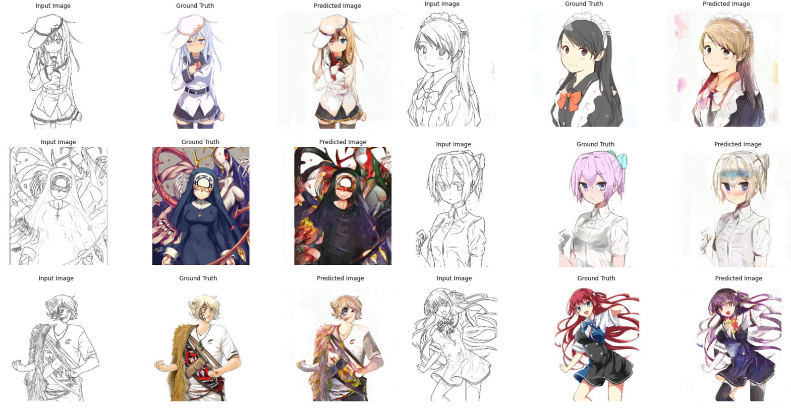
Outputs from the Generator model after 150 epochs (Gif made by Author)

This article is a part of the Gans-Series published by me on TowardsDataScience Publication on Medium. If you do not know what GANs are or if you have an idea about it but wish to quickly go over it again, I highly recommend you read the previous article which is just a 7 minutes long read and provides a simple understanding of GANs for people who are new to this amazing domain of Deep Learning.

As you can tell from the gif shown above, this article is going to be all about learning how to create a Conditional GAN to predict colorful images from the given black and white sketch inputs without knowing the actual ground truth.

A little bit of need-to-know stuff before bringing on the coding mode…

Sketch to Color Image generation is an image-to-image translation model using Conditional Generative Adversarial Networks as described in the original paper by Phillip Isola, Jun-Yan Zhu, Tinghui Zhou, Alexei A. Efros 2016, Image-to-Image Translation with Conditional Adversarial Networks.

When I first came across this paper, it was amazing to see such great results shown by the authors and the fundamental idea was amazing on its own too.

APPLICATIONS

There are a lot of application scenarios of Conditional GANs that are depicted in the original paper by the authors. Some of which are listed below.

• Map to Aerial Photos and vice versa
• Cityscapes to Photos
• Building Facades Labels to Photos
• Daylight Photos to Night
• Photo Inpainting
• Sketch to Color Images (the one which we are going to build in this article)

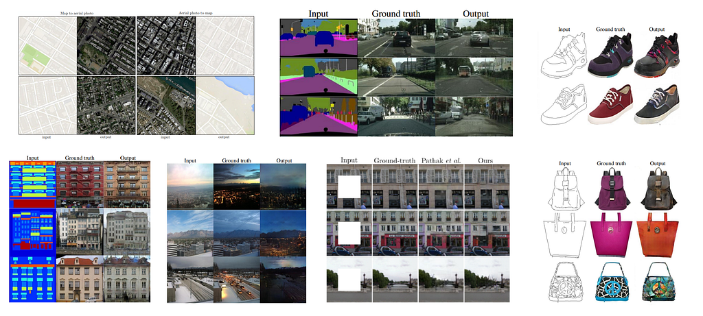
Images were taken from Phillip Isola, Jun-Yan Zhu, Tinghui Zhou, Alexei A. Efros 2016, Image-to-Image Translation with Conditional Adversarial Networks

We are going to build a Conditional Generative Adversarial Network which accepts a 256x256 px black and white sketch image and predicts the colored version of the image without knowing the ground truth. The model will be trained on the Anime Sketch-Colorization Pair Dataset available on Kaggle which contains 14.2k pairs of Sketch-Color Anime Images.

When I trained the model on my system, I ran the model for 150 epochs which took approximately 23 hours on a single GeForce GTX 1060 6GB Graphic Card and 16 GB RAM. After all that hard work and patience, the results were totally worth it!

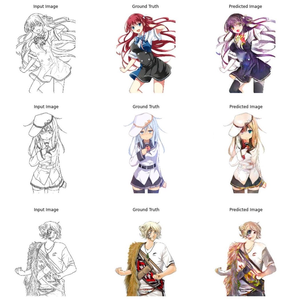
Outputs of the Trained Generator Model (Image by Author)

Let’s get to the interesting part now…

To build this model I have used TensorFlow 2.x and most of the code is based on their awesome tutorial on Pix2Pix for CMP Facade Dataset which predicts building photos from facade labels. TensorFlow tutorials are a good way to understand the framework and work on some well-known projects. I highly recommend you to go through all the tutorials on the website — https://www.tensorflow.org/tutorials.

REQUIREMENTS

To build this model, there are some basic requirements that you need to install on your system in order for it to work properly.

• Python 3.6 and above
• pip 19.0 or later
• Windows 7 or later (64-bit)
• Microsoft Visual C++ Redistributable for Visual Studio 2015, 2017 and 2019
• Tensorflow 2.2 and above
• GPU support requires a CUDA®-enabled card

If you are planning on using any cloud environments like Google Colab, you need to keep in mind that the training is going to take a lot of time as GANs are computationally quite heavy to run. Google Colab has an absolute timeout of 12 hours which means that the notebook kernel is reset so you’ll need to consider some points like mounting the Google Drive and saving checkpoints after regular intervals so that you can continue training from where it left off before the timeout.

DOWNLOADING THE DATASET

Download the Anime Sketch-Colorization Pair Dataset available on Kaggle and save it to a folder directory. The root folder will contain folders colorgram , train , and val . For everyone’s convenience let us call the path to the root folder as path/to/dataset/ .

Once the basic requirements are checked and the dataset is downloaded to your machine, it’s time for you to get into coding your very own Conditional GAN.

Before we jump right into it, note that the code which I’m going to provide shouldn't just be copied and pasted from here if you wish to understand the basic working behind it. And do not hesitate to ask your queries because that’s how things are learned — by asking.

FINALLY, THE CODE!

First, let’s initialize the parameters to configure the training of the model. As stated earlier, we will be using the TensorFlow framework so we’ll need to import it by using import tensorflow as tf .

The os module is used to interact with the Operating System. We are going to use this for accessing and modifying the path variables to save checkpoints during training. The time module lets us display relative time and hence, we can check how much time each epoch took during the training.

matplotlib is another cool python library which we will be using to plot and show images.

BUFFER_SIZE is used when we shuffle the data samples while training. Higher the value of this more will be the degree of shuffling, and hence, higher will be the accuracy of the model. But with large data, it takes a lot of processing power to shuffle the images. For my system with Intel(R) Core(TM) i7–8750H CPU and 16 GB of RAM, it was possible to set it equal to the size of the train dataset samples i.e. 14,224.

NOTE: The highest efficiency of shuffle() is when you set buffer_size equal to the size of data samples. This way it takes all the samples [in this case 14,224] in the primary memory and chooses a random one from those. If you set it to 10, it’ll take the 10 samples in the memory and choose a random one from those 10 samples and then repeat it for other remaining examples. So, check you machine capabilities and find out the sweet spot.

BATCH_SIZE is used to divide the dataset into mini-batches for training. The higher this value is, the faster will be the process of training. But as you might have guessed already, higher batch size means a higher load on the machine.

import tensorflow as tf

import os
import time

from matplotlib import pyplot as plt

# Change PATH variable to absolute/ relative path to the images directory on your machine which contains the train and val folders
PATH = '../path/to/data' 

# Change these variables as per your need
EPOCHS = 100
BUFFER_SIZE = 14224
BATCH_SIZE = 4
IMG_WIDTH = 256
IMG_HEIGHT = 256

Now, if you take a look at the dataset, you have a single image of size 1024x512 px for one entry which has a colored image of size 512x512 px in the left and a black and white sketch image of size 512x512 px in the right.

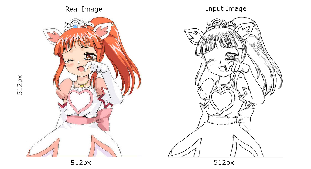
Visualizing Data (Image from the Anime Sketch-Colorization Pair Dataset)

We will define a function load() that takes the image path as a parameter and returns an input_image which is the black and white sketch that we’ll give as an input to the model, and real_image which is the colored image that we want.

def load(image_file):
    image = tf.io.read_file(image_file)
    image = tf.image.decode_png(image)

    w = tf.shape(image)[1]

    w = w // 2
    real_image = image[:, :w, :]
    input_image = image[:, w:, :]

    input_image = tf.cast(input_image, tf.float32)
    real_image = tf.cast(real_image, tf.float32)

    return input_image, real_image

Preprocessing

Now that we have the data loaded, we need to do some preprocessing in order to prepare the data for the model.

Given below are a few easy functions used for this purpose.

resize() function is used to return the images as 286x286 px. This is done in order to have a uniform image size if by chance there is a differently sized image in the dataset. And decreasing size from 512x512 px to half of it also helps in speeding up the model training as it is computationally less heavy.

random_crop() function returns the cropped input and real images which have the desired size of 256x256 px.

normalize() function, as the name suggests, normalizes images to [-1, 1].

def resize(input_image, real_image, height, width):
    input_image = tf.image.resize(input_image, [height, width],
                                method=tf.image.ResizeMethod.NEAREST_NEIGHBOR)
    real_image = tf.image.resize(real_image, [height, width],
                               method=tf.image.ResizeMethod.NEAREST_NEIGHBOR)

    return input_image, real_image

def random_crop(input_image, real_image):
    stacked_image = tf.stack([input_image, real_image], axis=0)
    cropped_image = tf.image.random_crop(
      stacked_image, size=[2, IMG_HEIGHT, IMG_WIDTH, 3])

    return cropped_image[0], cropped_image[1]

def normalize(input_image, real_image):
    input_image = (input_image / 127.5) - 1
    real_image = (real_image / 127.5) - 1

    return input_image, real_image

@tf.function()
def random_jitter(input_image, real_image):
    input_image, real_image = resize(input_image, real_image, 286, 286)
    input_image, real_image = random_crop(input_image, real_image)

    if tf.random.uniform(()) > 0.5:
        input_image = tf.image.flip_left_right(input_image)
        real_image = tf.image.flip_left_right(real_image)

    return input_image, real_image

In the random_jitter() function shown above, all the previous preprocessing functions are put together and random images are flipped horizontally. You can see what the preprocessing of data returns from images given below.

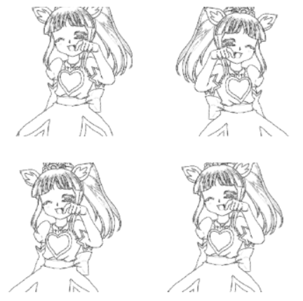
Preprocessed Images (Image by Author)

Loading the Train & Test Data

load_image_train() function is used to put together all the previously seen functions and output the final preprocessed image.

tf.data.Dataset.list_files() collects the path to all the png files available in the train/ folder of the dataset. Then the collection of these paths is mapped through and every path is sent individually as an argument to the load_image_train() function which returns the final preprocessed image and adds it to the train_dataset .

Finally, this train_dataset is shuffled using the BUFFER_SIZE and then divided into mini-batches as discussed earlier.

def load_image_train(image_file):
    input_image, real_image = load(image_file)
    input_image, real_image = random_jitter(input_image, real_image)
    input_image, real_image = normalize(input_image, real_image)

    return input_image, real_image
    
train_dataset = tf.data.Dataset.list_files(PATH+'\\train\\*.png')
train_dataset = train_dataset.map(load_image_train, num_parallel_calls=tf.data.experimental.AUTOTUNE)
train_dataset = train_dataset.shuffle(BUFFER_SIZE).batch(BATCH_SIZE)

To load the test dataset, we will use a similar process except for a small change. Here we will omit the random_crop() and random_jitter() functions as there is no need to do this for testing the results. Also, we can omit to shuffle the dataset for the same reason.

def load_image_test(image_file):
    input_image, real_image = load(image_file)
    input_image, real_image = resize(input_image, real_image,
                                   IMG_HEIGHT, IMG_WIDTH)
    input_image, real_image = normalize(input_image, real_image)

    return input_image, real_image
  
test_dataset = tf.data.Dataset.list_files(PATH+'\\val\\*.png')
test_dataset = test_dataset.map(load_image_test)
test_dataset = test_dataset.batch(BATCH_SIZE)

Building the Generator Model

Let us build the generator model now which takes an input black and white sketch image of 256x256 px and outputs an image that hopefully resembles the colored ground truth image in the training dataset.

The Generator model is a UNet Architecture Model and has skip connections to other layers than the intermediate one. Take note that it becomes complex to design such an architecture as the output and input shapes need to match to the connected layers, so design this carefully.

The downsampling stack of layers has Convolutional layers which result in a decrease in the size of the input image. And once the decreased image goes through the upsampling stack of layers which has kind of “reverse” Convolutional layers, the size is restored back to 256x256 px. Hence, the output of the Generator Model is a 256x256 px image with 3 output channels.

OUTPUT_CHANNELS = 3

def downsample(filters, size, shape, apply_batchnorm=True):
    initializer = tf.random_normal_initializer(0., 0.02)

    result = tf.keras.Sequential()
    result.add(
      tf.keras.layers.Conv2D(filters, size, strides=2, padding='same', batch_input_shape=shape, 
                             kernel_initializer=initializer, use_bias=False))

    if apply_batchnorm:
        result.add(tf.keras.layers.BatchNormalization())

    result.add(tf.keras.layers.LeakyReLU())

    return result

def upsample(filters, size, shape, apply_dropout=False):
    initializer = tf.random_normal_initializer(0., 0.02)

    result = tf.keras.Sequential()
    result.add(
    tf.keras.layers.Conv2DTranspose(filters, size, strides=2, batch_input_shape=shape,
                                    padding='same',
                                    kernel_initializer=initializer,
                                    use_bias=False))

    result.add(tf.keras.layers.BatchNormalization())

    if apply_dropout:
        result.add(tf.keras.layers.Dropout(0.5))

    result.add(tf.keras.layers.ReLU())

    return result

def buildGenerator():
    inputs = tf.keras.layers.Input(shape=[256,256,3])

    down_stack = [
        downsample(64, 4, (None, 256, 256, 3), apply_batchnorm=False), # (bs, 128, 128, 64)
        downsample(128, 4, (None, 128, 128, 64)), # (bs, 64, 64, 128)
        downsample(256, 4, (None, 64, 64, 128)), # (bs, 32, 32, 256)
        downsample(512, 4, (None, 32, 32, 256)), # (bs, 16, 16, 512)
        downsample(512, 4, (None, 16, 16, 512)), # (bs, 8, 8, 512)
        downsample(512, 4, (None, 8, 8, 512)), # (bs, 4, 4, 512)
        downsample(512, 4, (None, 4, 4, 512)), # (bs, 2, 2, 512)
        downsample(512, 4, (None, 2, 2, 512)), # (bs, 1, 1, 512)
    ]

    up_stack = [
        upsample(512, 4, (None, 1, 1, 512), apply_dropout=True), # (bs, 2, 2, 1024)
        upsample(512, 4, (None, 2, 2, 1024), apply_dropout=True), # (bs, 4, 4, 1024)
        upsample(512, 4, (None, 4, 4, 1024), apply_dropout=True), # (bs, 8, 8, 1024)
        upsample(512, 4, (None, 8, 8, 1024)), # (bs, 16, 16, 1024)
        upsample(256, 4, (None, 16, 16, 1024)), # (bs, 32, 32, 512)
        upsample(128, 4, (None, 32, 32, 512)), # (bs, 64, 64, 256)
        upsample(64, 4, (None, 64, 64, 256)), # (bs, 128, 128, 128)
    ]

    initializer = tf.random_normal_initializer(0., 0.02)
    last = tf.keras.layers.Conv2DTranspose(OUTPUT_CHANNELS, 4,
                                           strides=2,
                                           padding='same',
                                           kernel_initializer=initializer,
                                           activation='tanh') # (bs, 256, 256, 3)

    x = inputs

    skips = []
    for down in down_stack:
        x = down(x)
        skips.append(x)

    skips = reversed(skips[:-1])

    for up, skip in zip(up_stack, skips):
        x = up(x)
        x = tf.keras.layers.Concatenate()([x, skip])

    x = last(x)

    return tf.keras.Model(inputs=inputs, outputs=x)

generator = buildGenerator()

You can take a look at the model summary which is given below.

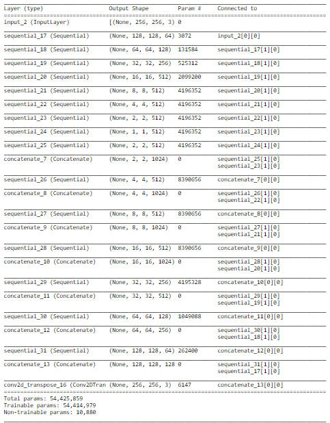
Model Summary for Generator Model (Image by Author)

Building the Discriminator Model

The primary purpose of the discriminator model is to find out which image is from the actual training dataset and which is an output from the generator model.

def downs(filters, size, apply_batchnorm=True):
    initializer = tf.random_normal_initializer(0., 0.02)

    result = tf.keras.Sequential()
    result.add(
      tf.keras.layers.Conv2D(filters, size, strides=2, padding='same', 
                             kernel_initializer=initializer, use_bias=False))

    if apply_batchnorm:
        result.add(tf.keras.layers.BatchNormalization())

    result.add(tf.keras.layers.LeakyReLU())

    return result

def buildDiscriminator():
    initializer = tf.random_normal_initializer(0., 0.02)

    inp = tf.keras.layers.Input(shape=[256, 256, 3], name='input_image')
    tar = tf.keras.layers.Input(shape=[256, 256, 3], name='target_image')

    x = tf.keras.layers.concatenate([inp, tar]) # (bs, 256, 256, channels*2)

    down1 = downs(64, 4, False)(x) # (bs, 128, 128, 64)
    down2 = downs(128, 4)(down1) # (bs, 64, 64, 128)
    down3 = downs(256, 4)(down2) # (bs, 32, 32, 256)

    zero_pad1 = tf.keras.layers.ZeroPadding2D()(down3) # (bs, 34, 34, 256)
    conv = tf.keras.layers.Conv2D(512, 4, strides=1,
                                kernel_initializer=initializer,
                                use_bias=False)(zero_pad1) # (bs, 31, 31, 512)

    batchnorm1 = tf.keras.layers.BatchNormalization()(conv)

    leaky_relu = tf.keras.layers.LeakyReLU()(batchnorm1)

    zero_pad2 = tf.keras.layers.ZeroPadding2D()(leaky_relu) # (bs, 33, 33, 512)

    last = tf.keras.layers.Conv2D(1, 4, strides=1,
                                kernel_initializer=initializer)(zero_pad2) # (bs, 30, 30, 1)

    return tf.keras.Model(inputs=[inp, tar], outputs=last)
  
discriminator = buildDiscriminator()

You can take a look at the model summary of the Discriminator given below. This is not as complex as the Generator model as it’s fundamental task is just to classify real and fake images.

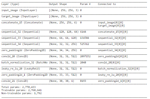
Discriminator Model Summary (Image by Author)

Loss Functions for the Models

As we have two models with us, we are going to require two different loss functions to calculate their loss independently.

The loss for the generator is calculated by finding the sigmoid cross-entropy loss of the output of the generator and an array of ones. This means that we are training it to trick the discriminator in outputting the value as 1, which means that it is a real image. Also, for the output to be structurally similar to the target image, we take L1 loss along with it. The value of LAMBDA is suggested to be kept 100 by authors of the original paper.

For discriminator loss, we take the same sigmoid cross-entropy loss of the real images and an array of ones and add it with the cross-entropy loss of the output images of the generator model and array of zeros.

loss_object = tf.keras.losses.BinaryCrossentropy(from_logits=True)

LAMBDA = 100

def generator_loss(disc_generated_output, gen_output, target):
    gan_loss = loss_object(tf.ones_like(disc_generated_output), disc_generated_output)

    l1_loss = tf.reduce_mean(tf.abs(target - gen_output))

    total_gen_loss = gan_loss + (LAMBDA * l1_loss)

    return total_gen_loss, gan_loss, l1_loss

def discriminator_loss(disc_real_output, disc_generated_output):
    real_loss = loss_object(tf.ones_like(disc_real_output), disc_real_output)

    generated_loss = loss_object(tf.zeros_like(disc_generated_output), disc_generated_output)

    total_disc_loss = real_loss + generated_loss

    return total_disc_loss

Optimizers

Optimizers are algorithms or methods used to change the attributes of your neural network such as weights and learning rates in order to reduce the losses. Adam Optimizer is one of the best ones to use, in most of the use cases.

generator_optimizer = tf.keras.optimizers.Adam(2e-4, beta_1=0.5)
discriminator_optimizer = tf.keras.optimizers.Adam(2e-4, beta_1=0.5)

Creating Checkpoints

As discussed earlier, cloud environments have a specific timeout which can interrupt the training process. Also, if you are using your local system, there may arise some cases where the training might be interrupted due to some reasons.

GANs take a very long time to train and are computationally expensive. So, it is best to keep saving checkpoints at regular intervals so that you can restore to the latest checkpoint and continue from there without losing the previously done hard work by your machines.

checkpoint_dir = './Sketch2Color_training_checkpoints'
checkpoint_prefix = os.path.join(checkpoint_dir, "ckpt")
checkpoint = tf.train.Checkpoint(generator_optimizer=generator_optimizer,
                                 discriminator_optimizer=discriminator_optimizer,
                                 generator=generator,
                                 discriminator=discriminator)

Displaying Output Images

def generate_images(model, test_input, tar):
    prediction = model(test_input, training=True)
    plt.figure(figsize=(15,15))

    display_list = [test_input[0], tar[0], prediction[0]]
    title = ['Input Image', 'Ground Truth', 'Predicted Image']

    for i in range(3):
        plt.subplot(1, 3, i+1)
        plt.title(title[i])
        plt.imshow(display_list[i] * 0.5 + 0.5)
        plt.axis('off')
    plt.show()

The above-given block of code is a basic python function which uses the pyplot module from matplotlib library to display the predicted images by the generator model.

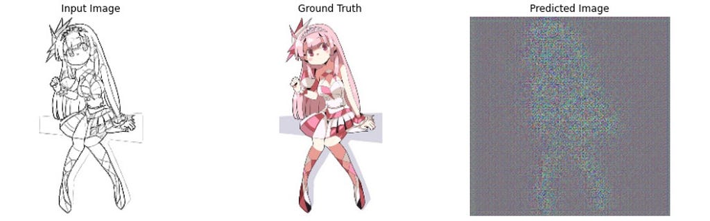
Displaying the predicted image by untrained Generator Model (Image by Author)

Logging the Losses

You can log the important metrics like losses in a file so that you can analyze it as the training progresses on tools like Tensorboard.

import datetime
log_dir="Sketch2Coloe_logs/"

summary_writer = tf.summary.create_file_writer(
  log_dir + "fit/" + datetime.datetime.now().strftime("%Y%m%d-%H%M%S"))

Train Step

A basic train step will consist of the following processes:

• The generator outputs a prediction
• The discriminator model is designed to have 2 inputs at a time. For the first time, it is given an input sketch image and the generated image. The next time it is given the real target image and the generated image.
• Now the generator loss and discriminator loss are calculated.
• Then, the gradients are calculated from the losses and applied to the optimizers to help the generator produce a better image and also to help discriminator detect the real and generated image with better insights.
• All the losses are logged using summary_writer defined previously using tf.summary .

@tf.function
def train_step(input_image, target, epoch):
    with tf.GradientTape() as gen_tape, tf.GradientTape() as disc_tape:
        gen_output = generator(input_image, training=True)

        disc_real_output = discriminator([input_image, target], training=True)
        disc_generated_output = discriminator([input_image, gen_output], training=True)

        gen_total_loss, gen_gan_loss, gen_l1_loss = generator_loss(disc_generated_output, gen_output, target)
        disc_loss = discriminator_loss(disc_real_output, disc_generated_output)

    generator_gradients = gen_tape.gradient(gen_total_loss,
                                          generator.trainable_variables)
    discriminator_gradients = disc_tape.gradient(disc_loss,
                                               discriminator.trainable_variables)

    generator_optimizer.apply_gradients(zip(generator_gradients,
                                          generator.trainable_variables))
    discriminator_optimizer.apply_gradients(zip(discriminator_gradients,
                                              discriminator.trainable_variables))

    with summary_writer.as_default():
        tf.summary.scalar('gen_total_loss', gen_total_loss, step=epoch)
        tf.summary.scalar('gen_gan_loss', gen_gan_loss, step=epoch)
        tf.summary.scalar('gen_l1_loss', gen_l1_loss, step=epoch)
        tf.summary.scalar('disc_loss', disc_loss, step=epoch)

Model.fit()

TensorFlow is an awesome, easy to use framework for training models. And one small command like model.fit() does the magic for us.

Unfortunately, it will not directly work over here as we have created two models that work together. But it is pretty easy to do this too.

Here we iterate over for every epoch and assign the relative time to start variable. Then we display an example of the generated image by the generator model. This example helps us visualize how the generator gets better at generating better-colored images with every epoch. Then we call the train_step function for the model to learn from the calculated losses and gradients. And finally, we check if the epoch number is divisible by 5 to save a checkpoint. This means that we are saving a checkpoint after every 5 epochs of training are completed. After this entire epoch is completed, the start time is subtracted from the final relative time to count the time taken for that particular epoch.

def fit(train_ds, epochs, test_ds):
    for epoch in range(epochs):
        start = time.time()

        for example_input, example_target in test_ds.take(1):
            generate_images(generator, example_input, example_target)
        print("Epoch: ", epoch)

        for n, (input_image, target) in train_ds.enumerate():
            print('.', end='')
            if (n+1) % 100 == 0:
                print()
            train_step(input_image, target, epoch)
        print()

        if (epoch + 1) % 5 == 0:
            checkpoint.save(file_prefix = checkpoint_prefix)

        print ('Time taken for epoch {} is {} sec\n'.format(epoch + 1,
                                                        time.time()-start))
    checkpoint.save(file_prefix = checkpoint_prefix)

Aah! Finally, here we are…

fit(train_dataset, EPOCHS, test_dataset)

All we have to do now is run this one line of code and wait for the Model to do its magic on its own. Well let’s not give the entire credit to the model, we have done a lot of hard work and it’s time to see the results.

Restoring the Latest Checkpoint

Before moving forward, we must restore the latest checkpoint available in order to load the latest version of the trained model before testing it on the images.

checkpoint.restore(tf.train.latest_checkpoint(checkpoint_dir))

Testing Outputs

This randomly selects 5 images from the test_dataset and inputs them individually to the Generator Model. Now the model is trained well enough and predicts near-perfect colored versions of the input sketch images.

for example_input, example_target in test_dataset.take(5):
    generate_images(generator, example_input, example_target)

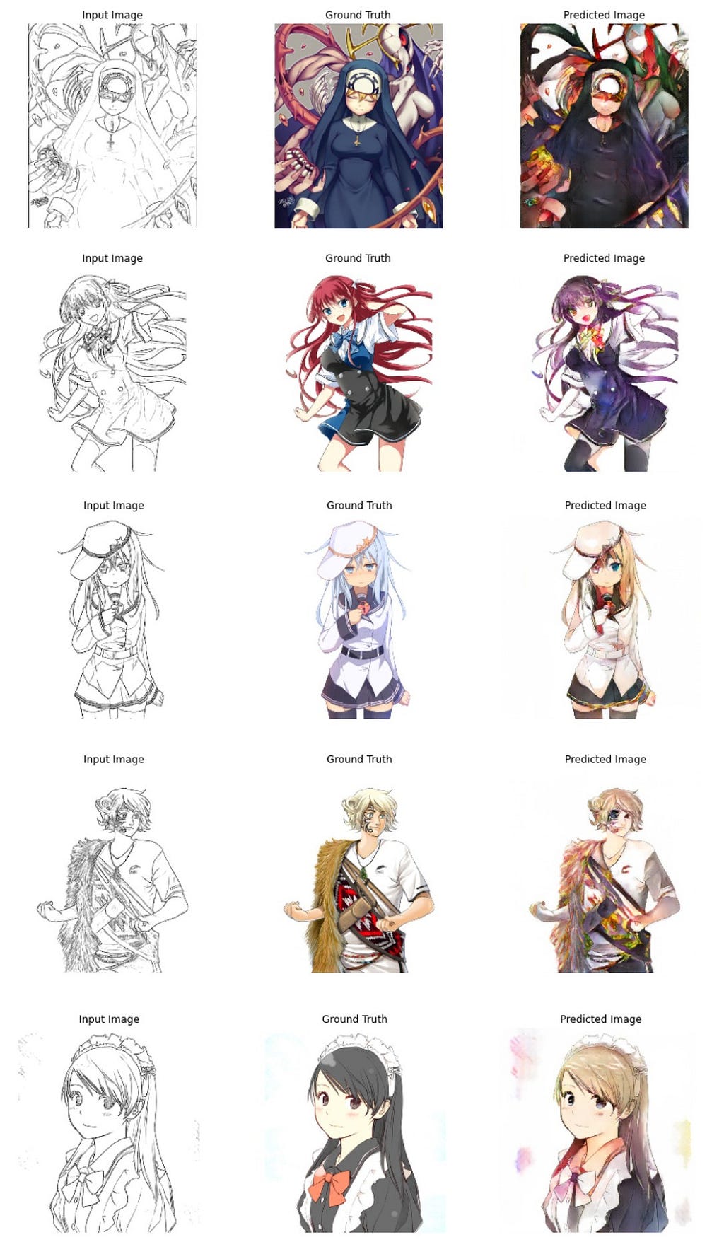
Outputs of Black and White Sketches after going through the trained Generator Model (Image by Author)

Saving the Model

Let’s not kill the model right after doing so much work, right?

A model shouldn’t end its life in a Jupyter Notebook!
- Rightly said by Daniel Bourke

It takes only a line of code to save the entire model as a .H5 file which is supported by Keras models.

generator.save('AnimeColorizationModelv1.h5')

CONCLUSION

So, that is it!

We have not only seen how a Conditional GAN works but also have successfully implemented it to predict colored images from the given black and white input sketch images.

You can go through the entire code and download it to see how it works on your system from my GitHub Repository.

Sketch to Color Image Generation Using Conditional GANs

If you face any problems, want to suggest some enhancements, or just want to leave a quick feedback, do not hesitate in contacting me through any medium that best suits you.

My Contact Information:

LinkedIn: https://www.linkedin.com/in/tejasmorkar/**
GitHub**: https://github.com/tejasmorkar
Twitter: https://twitter.com/TejasMorkar